How does a waveguide work
Pieter-Tjerk de Boer, PA3FWM web@pa3fwm.nl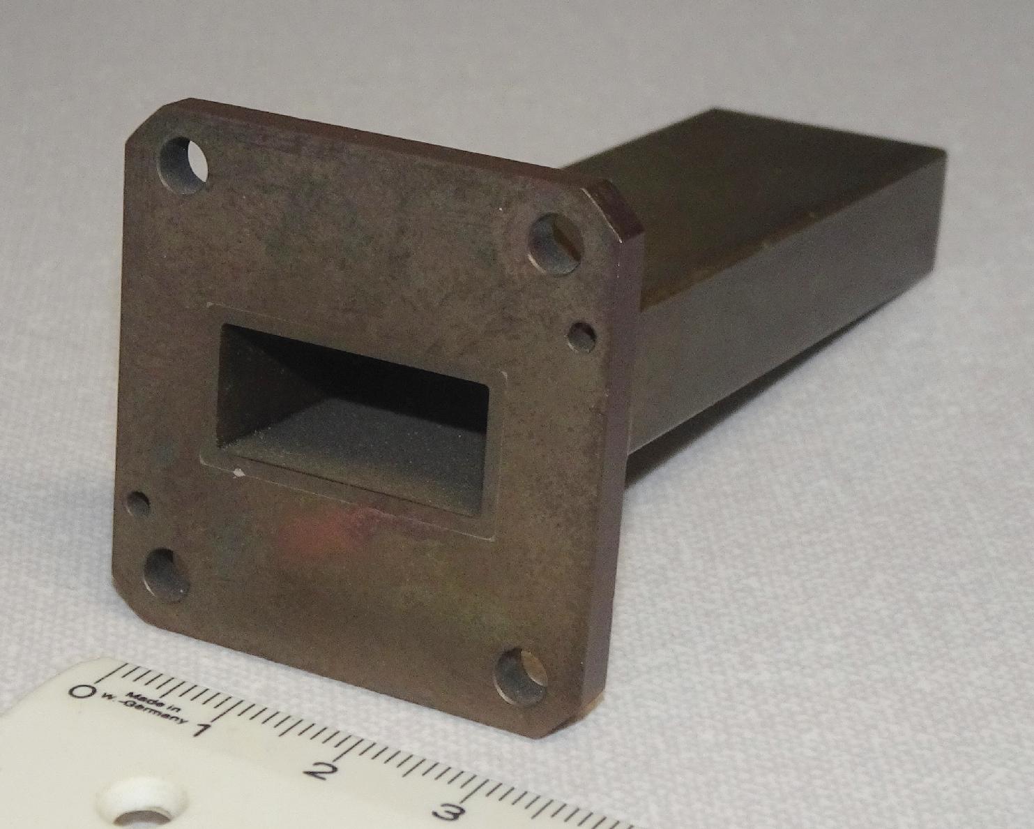
(This is an adapted version of an article I wrote for the Dutch amateur radio magazine Electron, January 2020.)
At microwave frequencies, instead of a coaxial cable often a waveguide is used: a hollow metal pipe through which radio signals propagate, with much less loss than in a coaxial cable. At first glance, it seems simple: if a radiowave can propagate in free space, it should be able to do so in a hollow pipe as well. But reality is a bit more complicated.
The problem
 What's the problem? Why can't a radiowave just pass through a waveguide without further ado?
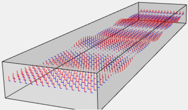
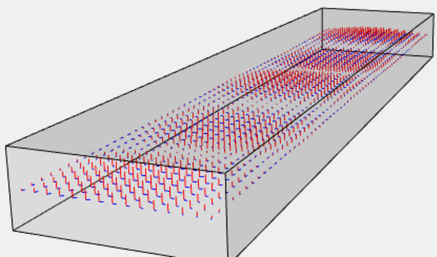
The figure shows a rectangular waveguide and a vertically polarized radio wave propagating
through the waveguide "away from the reader".
The red lines represent the electric field and the blue lines the magnetic field.
The electric field is vertical, the magnetic field horizontal, and both are at right angles to the
direction of propagation, as they should in a radiowave.
What's the problem? Why can't a radiowave just pass through a waveguide without further ado?
The figure shows a rectangular waveguide and a vertically polarized radio wave propagating
through the waveguide "away from the reader".
The red lines represent the electric field and the blue lines the magnetic field.
The electric field is vertical, the magnetic field horizontal, and both are at right angles to the
direction of propagation, as they should in a radiowave.
What goes wrong here is that there is a vertical electric field (red lines) at the left and right walls of the waveguide. That's not allowed. Just like a voltage cannot exist across a (perfect) conductor (one would short-circuit the voltage source), an electric field cannot exist along the surface of a conductor; such a field would be "short-circuited" as well. An electric field can only exist near a conductor if it is perpendicular to the conductor. In our example this is the case at the top and bottom walls of the waveguide, but not at the left and right walls.
For the magnetic field, the rules are exactly opposite: near a conductor a magnetic field is allowed to point along the conductor, but not perpendicular to it. Again we see that this condition is satisfied at the top and bottom walls, but not at the left and right walls.
So, we have to find a solution which on the one hand behaves as radiowave in the interior of the waveguide, but on the other hand satisfies the boundary conditions at its walls. One can do this with a lot of math, resulting in a large number of possible solutions, only one of which is relevant in practice. Books that don't dive into the math usually don't go beyond a sketch of the resulting field lines of that single useful solution, without explaining why. I'd like to find a middle course here: explain without mathematics how that solution is composed.
Two diagonal waves
 As a start, let's simplify the picture.
Instead of drawing a waveguide with lots of arrows, we'll from now on only draw a top view.
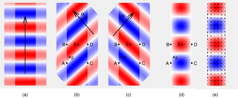
See figure (a), showing the top view of the same situation as the previous drawing.
We'll for now limit ourselves to the electric field and now use colour for the sign:
red for positive (upward in the previous drawing), blue for negative (downward).
We see a nice wave propagating upward: upward in this figure is what was "away from
the reader" in the previous drawing.
And again we see that this wave is not zero at the left and right walls of the waveguide.
As a start, let's simplify the picture.
Instead of drawing a waveguide with lots of arrows, we'll from now on only draw a top view.
See figure (a), showing the top view of the same situation as the previous drawing.
We'll for now limit ourselves to the electric field and now use colour for the sign:
red for positive (upward in the previous drawing), blue for negative (downward).
We see a nice wave propagating upward: upward in this figure is what was "away from
the reader" in the previous drawing.
And again we see that this wave is not zero at the left and right walls of the waveguide.
Now let's rotate the wave a bit, see figure (b), so it is propagating in a diagonal direction. The wave seems to magically go through the walls of the waveguide, but we'll fix that later. For now it is important to observe that this wave is 0 at some spots on the walls, such as points A and B on the left wall and points C and D on the right wall. Between A and B, and between C and D, it is not zero, so the problem has not been solved yet.
Next, take a second diagonal wave, propagating under the same angle but to top right rather than top left, as in figure (c). Also this wave is zero at points A, B, C and D, and not in between. However, while the wave in figure (b) was positive (red) between points A and B, the wave in figure (c) is negative (blue) there.
If we now add the waves from figures (b) and (c), we get figure (d). We see that the result is not just zero at points A and B itself, but also at all other points on this wall. That is because contribution of (b) is equally large but has opposite sign as the contribution of (c). In the same way, the addition also gives zero everywhere on the right wall. So, we can conclude that the sum of both diagonal waves satisfies the boundary conditions!
At points in the interior of the waveguide, away from the walls, the diagonal waves do not cancel. For example, consider point E: there they both are positive, and so is their sum; or point F, where one is strongly negative while the other is weakly positive, resulting in a weakly negative sum.
In figures (b) and (c), the diagonal waves seemed to magically cross the waveguide walls. That is nonsense of course, and now that we know that both diagonal waves must be present simultaneously, we can understand what is happening in reality: one diagonal wave, reflected off the wall of the waveguide, gives the other diagonal wave, and vice versa. The waves effectively bounce back and forth. That's why I didn't draw a field outside the waveguide in figure (d).
Animations of these figures can be found elsewhere on this website, at ../tools/waveguide.html.
Cut-off frequency
Having the two diagonal waves cancel each other does not happen just like that. It only works if both diagonal waves propagate at the correct angle and have the right phase difference. If the phase is chosen differently, they won't cancel everywhere on the wall; and if the angle is different, points A and C, and B and D, are not aligned and it won't work out either. Just give it a try on a piece of scrap paper!The propagation angle, denoted α in the figure, depends both on the wavelength and the width of the waveguide. The wider the waveguide, or the smaller the wavelength, the smaller α becomes. And that makes intuitive sense: very small waves propagating in a very big waveguide should hardly notice the waveguide and propagate almost undisturbed straight ahead.
On the other hand, when the waveguide gets smaller, or the wavelength longer, α becomes larger and can reach 90 degrees. For even larger wavelengths our solution no longer exists: it is then no longer possible to construct a solution which satisfies the boundary conditions everywhere. This happens when the waveguide is narrower than half a wavelength. Thus, every waveguide has a cut-off frequency: frequencies below that cannot propagate through the waveguide.
The WR90 waveguide shown at the top of the page has an internal width of 22.86 mm; that is 0.90 inch, hence the name WR90. This is half the wavelength of the cut-off frequency, so we calculate the cut-off to be at 6.56 GHz. In practice, WR90 is used between 8.2 and 12.4 GHz.
Speed(s)
As the waves do not go through the waveguide in a straight line, but bounce back and forth, they take a detour. Their speed remains the speed of light, so the detour means that they need more time: their net speed is lower than in free space. As the frequency decreases, the angle α increases, and so does the detour. At the cut-off frequency, the net speed becomes 0.That's not the complete story though. Have a look at figure (d): in the center of the waveguide we see an alternation of maximums and minimums, or peaks and troughs. If we measure the distance between two consecutive maximums, we find that this is more than that of the wave in free space (figure (a)). This is really odd, because at the same frequency, a larger wavelength would imply a higher speed. Eh, higher? Didn't we just also conclude that the speed in the waveguide would be lower? Furthermore, wasn't it Einstein who forbids exceeding the speed of light?
 As it turns out, the higher speed in figure (d) is deceptive.
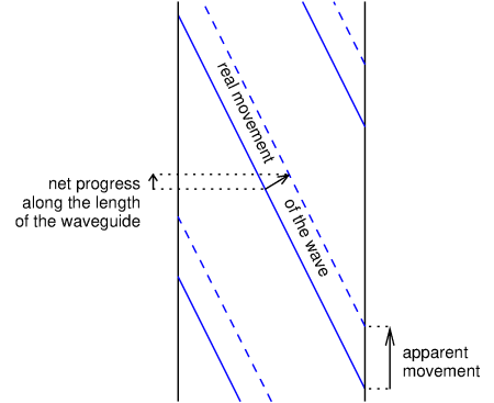
See the next figure.
We see a couple of wavefronts sketched as blue solid lines, and the same wavefronts
a little bit later as dashed lines: they move diagonally to top right, like in the previous figure (c).
We see that the net progress along the waveguide is indeed much less than the
real distance moved by the waves.
But if we look at where the wave "washes ashore" at the waveguide's right wall ,
then we see that this point as moved over a larger distance.
But this point is deceptive: there is not really anything actually moving along the wall!
Compare this to closing a pair of scissors: the apparent point where the blades reach each
other, moves much faster than the actual motion of the blades.
As it turns out, the higher speed in figure (d) is deceptive.
See the next figure.
We see a couple of wavefronts sketched as blue solid lines, and the same wavefronts
a little bit later as dashed lines: they move diagonally to top right, like in the previous figure (c).
We see that the net progress along the waveguide is indeed much less than the
real distance moved by the waves.
But if we look at where the wave "washes ashore" at the waveguide's right wall ,
then we see that this point as moved over a larger distance.
But this point is deceptive: there is not really anything actually moving along the wall!
Compare this to closing a pair of scissors: the apparent point where the blades reach each
other, moves much faster than the actual motion of the blades.
(There is another way of looking at this, in which the lower real speed is the so-called "group velocity" and the apparent higher speed is the "phase velocity". But that's a topic for another occasion.)
 The apparenty high speed does play a practical role when measurements are done using a
so-called "slotted line", as pictured.
Such an instrument contains a piece of waveguide with a slot along its length.
A detector sticks into the waveguide through the slot and can be moved along the waveguide.
This can be used to measure standing waves in the waveguide.
The apparenty high speed does play a practical role when measurements are done using a
so-called "slotted line", as pictured.
Such an instrument contains a piece of waveguide with a slot along its length.
A detector sticks into the waveguide through the slot and can be moved along the waveguide.
This can be used to measure standing waves in the waveguide.
The magnetic field
 So far, we have only looked at the electric field, but of course there is also a magnetic field.
This has been depicted as arrows in the earlier figure (e).
So far, we have only looked at the electric field, but of course there is also a magnetic field.
This has been depicted as arrows in the earlier figure (e).
How did we find out how the magnetic field is arranged? For example, look at point E in figure (b). The wave moves to top left, the electric field is perpendacular to the screen, so the magnetic field must point to top right. Similarly, the magnetic field in point E of figure (c) points to lower right. Adding them gives a magnetic field pointing purely to the right, as we indeed see in figure (e) at that location.
Thus, we see that the magnetic field near the waveguide's wall is indeed nicely parallel to the wall, and thus satisfies the boundary condition mentioned earlier.
The final result is depicted here, again with red arrows for the electric field and blue for the magnetic field, just like in the first drawing on this page.
Other modes
The solution described above is called the TE10. TE means Transverse Electric: the electric field is perpendicular to the waveguide's length. The 1 means there is one maximum along the width of the waveguide, and the 0 means that at every height in the waveguide the field is the same.There exist other modes, corresponding to other angles for the diagonal waves, and/or having not a transversal electric but a transversal magnetic field. In a rectangular waveguide all those other modes have a higher cut-off frequency than the TE10 mode.
In practice, waveguides are used at frequencies in which only one mode works, so between the cut-off frequency of TE10 and the first higher mode. At higher frequencies multiple modes are possible, and they all propagate at a different speed. As a consequence, the signal would arrive from the waveguide several times with different delays, which is not desirable.
Eiffel tower
As noted in the beginning, waveguides are usually used at microwave frequencies. We now know why: the waveguide must be at least half a wavelength wide, which would be unpractical at lower frequencies. Coaxial cables are more convenient there. Furthermore, the losses in a coaxial cable are generally acceptably low at lower frequencies.But sometimes waveguides are used at lower frequencies. A nice example was used between 1962 and 2011 in the Eiffel tower: a waveguide of about 300 m long, connecting the TV transmitters at the foot of the tower to the antennas on top. For frequencies just above 470 MHz the waveguide must be at least 33 cm wide; in reality it was about half a meter. An impressive picture can be found at http://www.stephanecompoint.com/41,,,20516.html [archived].
Upon the switchover to digital TV transmission, the waveguide has been replaced by a coaxial cable. What happened to the waveguide? It has been removed from the tower with quite some effort (see http://www.stephanecompoint.com/11,688.html [archived]), and I guess most of it has been molten and recycled, given the world-wide demand for copper. Except for a few small fragments: those have been handed out as souvenirs to the guests of a VIP evening on the occasion of the switch to digital television... https://sfxpp.satellifacts.com/news/clin-d-aeil/clin-d-aeil-soiree-vip-a-la-tour-eiffel-pour-une-nuit-sans-tele-n-oubliez-pas-durex (formerly https://www.satellifax.com/fr/tour/news/187842/ ).